


Logistic Regression


Logistic Regression is probably the first classification algorithm that is introduced to those who step into the world of Machine Learning.
Introduction
Logistic Regression is one of the most popular and powerful classification techniques. I personally think logistic regression can be considered as a bridge between the world of Machine Learning and Deep Learning. After all, logistic regression is just a neural network of one layer.
But how does logistic regression work? How does the math behind it makes it one of the most powerful classification algorithms that lays a foundation for the state-of-the-art neural networks? Before getting into logistic regression, it is necessary to understand that logistic regression is basically a linear regression that is clothed in a non-linear function known as sigmoid function. Linear Regression is another model which basically outputs a continuous value.
Math behind Linear Regression
Let’s understand the math behind it. A linear regression with one independent variable can be defined as:
![]()
Where,
- Y: is the output, a numerical continuous value , also known as the dependent variable
- X: is a dependent variable which is also known as feature vector
- W^T: is the weight vector which influences the contribution of the feature vector X to determine the decision boundary
- b: known as the bias value is a constant value which allows the activation to be shifted to the right or left, to better fit the data. You can think of the bias as a measure of how easy it is to get a node fire.
Activation Function
What if the task is to classify whether an image is of a dog or a cat, or whether a person has disease or not, we want answers in yes or not. In other words, we want a model which tells us the probability of a data point belonging to a particular class. For e.g., given an image of a dog, we want the model to predict that this is an image of a dog with more confidence than to predict it as a cat.
This is where the sigmoid activation function comes into play. When you pass the output of a linear regression into a sigmoid function, it becomes a logistic regression:
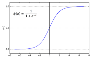
![]()
ŷ is the predicted value of the model.
The main reason of using a sigmoid function is because its value exists between 0 and 1. Therefore, it is especially used for models where we have to predict the probability as an output. Since the probabilities of anything exist only between the range of 0 and 1, sigmoid is the right choice.
If z is large, σ(z) tends to 1, while if z is small, σ(z) tends to 0.
Loss Function
Let’s define the loss function for logistic regression. Loss function basically means how good is your model is. In other words, it determines how close is the predicated value of the model to the actual value.
Let’s denote the loss function as l(ŷ,y), where ŷ is the predicted value and y is the actual value. Like regression, you cannot use squared error i.e. ![]() because when you learn the parameters w and b, the optimization problem becomes non-convex i.e. it has multiple local optimum values. This makes the gradient descent useless since it will get stuck at some local minima and miss the global minima.
because when you learn the parameters w and b, the optimization problem becomes non-convex i.e. it has multiple local optimum values. This makes the gradient descent useless since it will get stuck at some local minima and miss the global minima.
To avoid that we use binary cross entropy as the loss function defined as:
![]()
Let’s refer to this loss function as l for simplicity from this point onwards.
- If y = 1, then l = -log ŷ , i.e. ŷ should be as big as possible.
- If y = 0, then l = -log(1- ŷ), we want (1- ŷ) to be large, in other words we want ŷ to be as small as possible.
Now that we have defined the loss function, let’s define the cost function which basically means loss function over the entire training set:
![]()
Optimization Algorithm
Our next step is to define our optimization algorithm. We will be using gradient descent here.
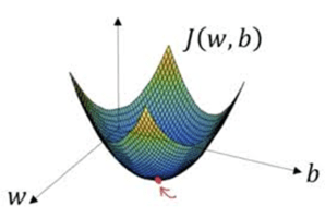
Gradient descent starts by randomly assigning values to w and b. The algorithm then calculates the slope and updates the variables until the slope is zero. In other words, updates are done, until we reach at the bottom of the function which is denoted by the red dot in above figure.
Since J(w,b) is a convex function, no matter where the initial values are,it will always get to the minimum point. Now that we have our cost function and optimization algorithm. We can apply forward and back propagation to find the optimum values of w and b.
-

By: Joel Jacob
I am a physicist turned Machine Learning Engineer. I started studying AI out of curiosity, little did I know that my curiosity would make my career. In my free time, I spend my time playing strategic games like chess and Age of Empires.
-
-
More from my site
 River For Online Machine Learning: An Example
 Software Project Selection Using Artificial Neural Networks
 Artificial Intelligence Vs. Human Intelligence
 Google Launches TensorFlow Machine Learning Framework for Graphical Data
 Gen – A New AI Programming Language by MIT
- River for Online Machine Learning in Python


Wonderful piece Joel. So intuitive. Waiting for the sequel 😊